Using Atmospheric Turbulence Models

LightLike models the optical effects of atmospheric turbulence using a standard wave optics technique, called in some references the "split-step" method.  The procedure is:

(1) Divide the propagation path into a number of subintervals.

(2) For each subinterval, compute the integrated turbulence strength based on a model of the continuous turbulence strength profile.

(3) For each subinterval, generate a "phase screen" whose optical path difference map, OPD(x,y), is a statistical realization that, in the mean, corresponds to the integrated turbulence strength.

(4) Position each screen at some point within its subinterval.

(5) Using Fresnel propagator formulas, propagate the optical beam from an initial plane to the first screen, apply that phase-screen distortion, propagate the result to the second screen, apply that phase-screen distortion, and repeat until the desired final plane is reached.

The time evolution of atmospheric turbulence is assumed to obey the Taylor frozen-flow hypothesis.  Thus, in addition to the above algorithm steps, we add the following:

(6) Model the time evolution of the turbulent propagation by shifting the phase screens relative to sources and sensors, by amounts consistent with the various transverse motion specifications that LightLike accepts.

As discussed previously, the Fresnel propagator used by LightLike is the spatial-frequency-domain form of the propagator.  Fast Fourier Transform algorithms are used to evaluate the two transform operations required by the propagator.

Propagation time delay effects are thoroughly and consistently accounted for:  all propagation time lags between screens are incorporated.  The various screens receive the wavefront in precise accord with the physical propagation time lag from screen to screen.  Thus, once given a full-path turbulence realization (a set of screens), all temporal and spatial correlations have correct contributions due to propagation lags between screens.

The phase distortion applied by any phase screen is expressed by

    u'(x,y) = u(x,y)*ei*k*OPD(x,y).

where u(x,y) is the complex field incident on the screen,  k is the wavenumber (2p / wavelength),  OPD(x,y) is the screen OPD in units of meters, and  u'(x,y) is the field exiting the screen.

The statistical realizations of the screens are generated in such a way as to reproduce the Kolmogorov statistics that describe locally homogeneous turbulence in the so-called inertial range.  In a later subsection, we discuss the algorithm for screen generation in somewhat more detail.  As a modification to the basic Kolmogorov statistics, the screen generation mechanism has options to impose an explicit inner or outer scale rolloff.  The inner scale modeling uses the "Hill bump" form of the turbulence spectrum.

Any number of phase screens may be used, but in practice the maximum used is typically 10 to 20.  LightLike allows arbitrary spacing of the screens;  uniform spacing or equal-strength spacing are frequently-used special cases.  Equal-strength spacing means that the full propagation distance is divided into subintervals whose nominal integrated-turbulence strengths are equal;  in this case, the lengths of the subintervals are unequal, unless the continuum strength profile is completely uniform.

LightLike has various options for specifying the phase screen strengths.  Usually the screen strengths are specified in terms of equivalent Cn2  values for the subintervals.  In general, Cn2  refers to the standard refractive-index structure parameter, which in LightLike always has the MKS units of m-2/3.

(Background note:  The Cn2  parameter is that constant which is defined by the Kolmogorov formula for the structure function of the refractive-index fluctuations:

    mean{ [n(r1) - n(r1+r)]2 } = Cn2 · r2/3

where n = refractive index, and r = separation of two points in the random medium.)

Specifying effective Cn2  values for LightLike phase screens

For wave-optics simulation, we typically know a model profile, Cn2(z), along the propagation path.  This may be uniform for near-horizontal paths, or may vary over orders of magnitude for a ground to high altitude path.  Several model profiles have been developed to describe the typical variation of Cn2  with vertical altitude, h, in the earth's atmosphere.  Some commonly used profiles are known by the names Hufnagel-Valley 5/7, Clear 1 Night, and SLC.  (For a discussion of these and profiles in general, see the review article by Beland).

A phase screen represents the integrated Cn2  strength over the distance corresponding to one subinterval.  This is indicated pictorially in the following diagram, where the symbol  ICn2  represents the integrated turbulence strength.

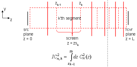
Based on the integrated Cn2 , we define an effective screen Cn2 as the path-averaged value:

    ( effective screen Cn,k2 ) = ICn,k2 / (zk - zk-1)

Whenever the LightLike user employs an input format that requests explicit values of screen Cn2 , the values are interpreted in the effective, or path-averaged sense just defined.  In other words, what LightLike does is to take an input value of screen Cn2 , and multiply it by the corresponding subinterval length (or screen "thickness") to obtain the integrated quantity that actually determines the screen OPD strength.

Phase-screen r0 values

Readers who are familiar with optical turbulence theory will realize that  ICn2  is closely related to the plane-wave r0 (Fried coherence length) quantity.  In fact, LightLike has one input format for specifying screen strengths that requests screen-r0 values.  Users who are familiar with this way of specifying screen strengths may prefer this input format to the Cn2-based formats.

Position of phase screens within the subintervals

In some LightLike input formats, the user can place the individual screens at arbitrary positions within their respective subintervals.  The best choice depends on the physical problem being modeled, and the turbulence path-weighting functions that are most important to the problem at hand.  Since several different weighting function are often significant in a physical problem, it is not always obvious what the optimum discrete positioning choice is.

In other LightLike input formats, the code internally decides where to place the screens within the designated subintervals.

Other phase screen parameters

In addition to the previously discussed strength and position parameters, the phase screen specifications contain numerous optional parameters.  Examples are screen transverse velocities, inner and outer scale lengths, and intensity transmission factors.  The availability and syntax of various options is documented in the section on the AcsAtmSpec function.  The remainder of the present section contains general remarks on several of the options.

Transverse velocities

Transverse velocities associated directly with the screens in the AcsAtmSpec function can be used in two ways.  If the velocities of target and platform motion are all specified by using TransverseVelocity library modules, then additional velocities specified explicitly as "screen velocities" should be interpreted as true-wind velocities.  LightLike will form the appropriate vector sums to obtain the relative motion of the nominal beam line with respect to the air mass.

There is a different approach to handling transverse velocity, which may be preferred by users who have some previous experience with "home-brewed" wave-optics simulation.  In many systems, one could dispense with LightLike's TransverseVelocity procedures, and simply precompute by hand the effective velocities with which the screens should be dragged, accounting for all target, platform, and true-wind velocities.  Then, these net pseudo-wind velocities could simply be inserted as the "screen velocities" in the AcsAtmSpec function.  These alternate approaches to handling transverse motion have been discussed at somewhat greater length in previous sections.

Inner and outer scales of turbulence

The optional inner and outer scale roll-offs are modifications to the pure Kolmogorov power-law spectrum of refractive index fluctuations.  The functional form and length of the outer scale depends in complicated ways on boundary conditions.  Modelers usually use a simple empirical rolloff known as the vonKarmann form, in which the Kolmogorov power law bends over and asymptotes to a constant at low spatial frequency.  The break point on a radian frequency scale is (1 / L0), where L0 is called the outer scale (see Andrews and Phillips, pp. 53ff.).  If desired, L0 can be specified on a screen-by-screen basis in AcsAtmSpec.  In many modeling problems, the outer scale is sufficiently larger than aperture or beam sizes so that L0 is effectively infinite.  If no outer scale specification is entered in AcsAtmSpec, it will be treated as infinite.

The inner scale modification of the Kolmogorov power spectrum is on a firmer theoretical and experimental footing than the outer scale.  When analysts explicitly include inner scale, it is often represented as a Gaussian rolloff factor at high spatial frequency, of the form

exp[-(K/Km)2], where K is radian spatial frequency, and the inner scale length is

l0 = 5.92/Km.   Although this form is more tractable for analytic calculations, the modern literature has established that a more accurate form of the spectral modification is the so-called "Hill bump" form (see Andrews and Phillips, pp. 53ff.).  In simulation, this functional form can be encoded with little extra trouble, and this option is available in the AcsAtmSpec function.  If desired, inner scale length can be specified on a screen-by-screen basis in AcsAtmSpec.  If no inner scale is specified, it will be treated as zero.  There is a practical limitation due to the discrete simulation mesh:  the propagation mesh spacing effectively determines an inner scale even though no explicit factor is entered into the spectrum formula from which the screens are constructed.

Transmission factors

Screen "transmission" implies intensity transmission to be associated with that screen or subinterval.  For most LightLike work, the screen transmission options are not used:  the library also provides overall transmission-factor modules, so it is unnecessary to decompose the transmission by screen.  The exception to this is if the LightLike thermal blooming capability is used, but then one must use a different input function anyway (MtbAtmSpec).

LightLike library modules used to specify turbulence

The LightLike subsystems used to model the optical effects of turbulence are AtmoPath or GeneralAtmosphere.  If the user prefers to get LightLike subsystems via the "sub-libraries", the two subsystems just named can be found inside the LightLike.Atmosphere sub-library.  As far as turbulence specification is concerned, there is no difference between AtmoPath and GeneralAtmosphere.  AtmoPath is a composite system that consists of GeneralAtmosphere plus two PropagationControllers.  For new LightLike users, we suggest the use of AtmoPath, which simplifies matters by automatically setting certain options.  The circumstances under which one wants to separately invoke GeneralAtmosphere and PropagationControllers are discussed in another Guide section.

In the present tutorial section, we explain the turbulence inputs in the context of the AtmoPath module.  The specifications are essentially the same in GeneralAtmosphere, when the user graduates to that level.  The diagram at right shows the interface of AtmoPath.  The module has a LightLike input and a LightLike output for each propagation direction.  Additionally, there are many parameters, and the ones directly relevant to turbulence specification are bracketed by the red bars.

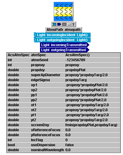
The first parameter, named atmSpec, has a unique data type, AcsAtmSpec.  This parameter carries all the information regarding the turbulence strength and distribution: the number of phase screens, their locations, strengths, inner scales, outer scales, and so forth.  In the sample at right, this information is entered in a setting expression that uses a special function from the LightLike library:

  AcsAtmSpec(...)

The name of the function should be entered just as shown, and the ellipsis replaced by a sequence of input arguments that has numerous options.  Several of the most useful argument syntax options of AcsAtmSpec are documented in detail in the next subsection.  From time to time, new options are added, and the more experienced and bold LightLike user may benefit from inspecting the source code file that contains all the options.

The second parameter, atmoSeed, is the random number seed used to initialize the sequence of phase screen statistical realizations.  This can be any allowed integer value.  This parameter allows the user to exactly reproduce a particular set of turbulence screens:  in this way, we can vary some overall system parameters while using exactly the same turbulence realizations.

The next relevant group of parameters stretches from xp1 to yt2.  These parameters specify the transverse spans of the phase screens.  As the system evolves, there may be relative motion between sources, medium, and sensors, causing the beams to sample different portions of the phase screens.  The relative motion of the screens is carried out internally by LightLike, based on transverse motion specifications defined by the user.  The "rectangular region"  (xp1,xp2, yp1,yp2)  defines the size of a screen at the platform end (should a screen be exactly at that z), while  (xt1,xt2, yt1,yt2)  defines the size of a screen at the target end (should a screen be exactly at that z).  The indices "1" and "2" here signify "min" and "max", respectively.  The sizes of screens at intermediate z locations are determined by linear interpolation from the "rectangular regions" at the two ends.  In previous sections on transverse motion, we explained in detail how the transverse motion during the full simulation is used to determine appropriate values for the screen "rectangular regions".  The numerical values entered as setting expressions in the above picture derive from an example discussed in that previous section.  The link just referenced should be reviewed in conjunction with the present one for full coverage of phase screen specifications.

The final turbulence parameter is screenDxy.  This is the mesh spacing of the phase screens.  We have set this spacing equal to the propdxy value, which is a typical choice, though not obligatory.  Based on screenDxy, LightLike may make some adjustment to the screen size because of FFT (Fast Fourier Transform) constraints.  For example, to determine one of the actual dimensions of the phase screen mesh,  (xp2-xp1)/screenDxy  will be rounded up to the nearest convenient integer for the FFT routines, so that the screens will usually be somewhat bigger than the user specifications (xp1,...).  

Use of AcsAtmSpec to specify turbulence parameters and path geometry

To enter turbulence specifications into a LightLike simulation, one uses the AcsAtmSpec function in a setting expression in AtmoPath or GeneralAtmosphere.  The mechanism was illustrated in the first parameter line in the preceding picture.  AcsAtmSpec has many different allowed sets of arguments.  (At the C++ code level, these options are referred to as different "constructors" or initialization functions.)  The following table documents several of the most useful syntax options.  From time to time, between official LightLike releases, new options are added by LightLike programmers to handle new special cases that are judged convenient or necessary.  The more experienced and bold LightLike user may benefit from inspecting the source code file that contains all the options.  After some of the cases documented below have been digested, the user can probably understand the multitudinous other allowed formats by inspecting the argument lists in the referenced source code file.

General rules

There are some general rules that apply to all argument list options (or at least to all cases where the item appears):

(1) In the table below, the data types of the arguments are prefixed to the arguments.  The purpose of doing this in the table is just to clarify whether the arguments are scalars or vectors:  when the user actually enters the setting expression in LightLike, the data type designators should be omitted.

(2) Argument lambda refers to a reference wavelength.

CAUTION:  the wavelength in question here may be, but is not necessarily, the wavelength of the propagating beam.  In the listed syntax options where it appears, lambda is the reference wavelength at which the r0s of the screens are defined.  The effective r0 of a screen will then depend on the propagating wavelength, but we want to define the screens only once, at some reference wavelength.

(3) Argument pathLength refers to the total propagation range from platform end to target end of the atmospheric module.  Note that screens are not necessarily located at the endpoints, so pathLength is frequently greater than the distance between first and last screens.

(4) The positions (z coordinates) of screens are defined with respect to LightLike's z-coordinate conventions.  The key facts are that z=0 is the platform end and z=L(propagation range) is the target end of the atmospheric propagation module into which AcsAtmSpec is inserted.

(5) Arguments that specify inner and outer scales, screen velocities, and screen transmissions have obvious default values.  The defaults are:  inner scale = 0.0, outer scale = infinity,  velocities = 0.0, and transmissions = 1.0.

To obtain the default values, the user should simply omit these arguments from the setting expression.  BUT, note that only a contiguous set of trailing arguments in a list may be omitted.

"Transmission" here implies intensity transmission to be associated with that screen or subinterval.  For most LightLike work, the screen transmission options are not used, because the library also provides overall transmission-factor modules.

(6) Some syntax options have height specifications, usually encoded as hPlatform  and hTarget.  In these cases the user can specify the turbulence strength in terms of a named turbulence profile, such as Clear-1, Clear-2, or HV57.  In these cases, h should be interpreted as height above mean sea level (AMSL), because the named Cn2 profile options such as "Clear-1" have their Cn2(h) functional forms defined in terms of height AMSL.  Additionally, when using the named profiles, the user must understand that the Clear-1 and Clear-2 profile functions are only defined for h ≥ 1230 m AMSL, where that height represents (approximately) the ground level altitude at the site where Clear-X data was collected.  If the user wishes to apply Clear-X to a physical problem where the ground altitude is different, then a reasonable approach would be to enter h_AMSL values into LightLike such that the altitude above ground level is preserved between the physical problem and the simulation specs.

(7) Particularly in the case of vector arguments, the user will find it most convenient to enter symbolic names for the arguments, elevate the arguments up the system hierarchy, and assign values to the vectors at that top level (i.e., in the Run Set Editor.

Actually, this holds for most scalar arguments as well:  the atmospheric specifications in general are quantities that we often wish to vary when exploring performance, so it is best to elevate those quantities to the Run Set level before assigning numerical values.

(8) As elsewhere in LightLike, physical units are MKS, unless explicitly specified otherwise.

Table of basic cases

Phase screen generation and execution time

Phase screen generation is done once, at the beginning of a simulation run.  For all subsequent time steps of the simulation run, the existing screens simply shift relative to sources and receivers.  This means that quite large screens can be used without much impact on the overall simulation wall-clock time, which is usually dominated by the Fresnel propagations.  If multiple runs (each with a different realization of the atmospheric screens) are included in a run set, then of course screens must be generated at the beginnning of each run.  The extreme case would be if a run set is constructed from N completely independent realizations, with only one time index per realization: in this case, the phase screen construction could dominate the execution time.  The earlier introduction to modeling transverse motion expanded on some of these issues.

Some phase screen construction details

In the previous discussion of determining the size of phase screens, we alluded to a second reason for making "oversize" screens.  We briefly discuss this second reason now.  A phase screen is a discrete, finite-span statistical realization of a 2-D random process that obeys a specified power spectral density law.  Currently, the standard LightLike library method of generating screens is the PSD-conditioned white-noise method.  The steps of this procedure are:  (a) use a standard random-number generator to create an uncorrelated (white) noise random process in the spatial-frequency domain;  (b) multiply that by the square root of the theoretical power spectral density (PSD);  (c) apply a suitably normalized discrete Fourier transform to obtain the space-domain realization of the correlated random process.  A consequence of this algorithm is that the random process it generates is periodic in both dimensions:  each edge matches up smoothly with the opposite edge.  This has an advantage, in that it makes endless scrolling of the screens possible, but it also means that there can be no overall phase tilt across the screen, which is physically incorrect.  In general, other lower-order spatial frequency modes, not just tilt, will also have less power than they should.

Low-order correction option ("locflag" in AtmoPath)

The low-order deficiency just described is often not serious, for several reasons.  First, it is typically practical to generate screens that are much bigger than the simulation apertures. As discussed previously, we usually want to generate oversize screens anyway because of relative motion considerations.  In this case, the tilt across the receiver aperture distance can be fairly well represented.  Secondly, for closed-loop adaptive optics systems, the lowest-order modes are the easiest to compensate, so one might argue that it is not very important to model them exactly.

On the other hand, to get accurate low-order results for uncompensated systems, users may want to invoke a modified screen-generation technique that AtmoPath makes available.  Inspection of AtmoPath's parameter list shows a parameter called locFlag, where "loc" stands for "low-order correction".  The default setting islocFlag = 0, which leaves the PSD-conditioned white-noise screens unchanged.  But, setting locFlag = 1 invokes a calculation that separately computes realizations of several low-order modes, and inserts a corresponding compensation into the phase screens that will be used for optical propagation.